Preprocessing data for data science (Part 1) :: Jinchuika

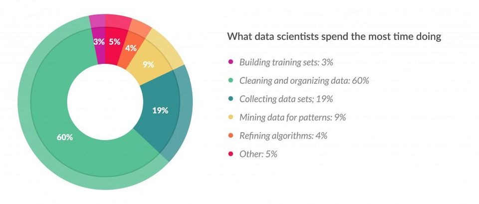
A study regarding data science jobs showed that 60% of the time spent by data scientists consists only on cleaning and organizing data. So in order to make the most out of our time, my data science fellas, in this four-part series we’ll se how to preprocess data like a boss, using the Pandas Python library and the preprocessing module from scikit-learn.

Pretty much everything we do in an AI algorithm are matrix operations. That means that every value must be represented in a numerical format and, ideally, one that optimizes the operations performance. Given that most datasets come in a very nonoptimal format, we must apply certain transformations in order to obtain the most ideal format. This process is called preprocessing.

Start of the cleaning data process

For this series of examples we’ll be using this interesting dataset of FIFA 19 players. This game allows players to create a custom character with different values for their stats like speed, weight, height, etc. We will create an algorithm for recommending the most ideal position (striker, central back, etc.) for that character based on those values and what we’ve learned from the rest of the football player base.

You can find all the code for this series in the GitHub repo.

As always, we’ll start by loading the data and do a basic exploration of it.

import pandas as pd
raw_df = pd.read_csv('data.csv')
# raw_df.info() # display all the columns and their data type

The very first thing to do is choosing what features could be useful for training the model. Let’s start by discriminating what features definitely won’t contribute and then choosing which ones could.

As rule of thumb, using unique non-numerical values is not useful since we want the model to generalize. So columns like ID and Name have to go. Features that are highly correlated to each other or are directly calculations don’t need to be included twice. For example, if we store the birth date, we don’t need to include the age since it is a result from the prior. In this case, Overall is the score resulting from the rest of the features, so there’s no need to have it.

Knowing what features influence the outcome of the objective one is a complex task. For the sake of this post lenght, we’ll arbitrarily pick some based on what we think impacts a player’s skill. Once the features are selected, let’s make a new data frame with only the colums we chose.

# it's useful to have the columns in a list you can modify easily
useful_columns = [
    'Age',
    'Preferred Foot',
    'Height',
    'Weight',
    'Agility',
    'Strength',
    'Dribbling',
    'Jumping',
    'Marking',
    'Interceptions',
    'Position', # I like to let my objective columns at the end
]
working_df = raw_df[useful_columns]
print(working_df.head())

   Age Preferred Foot Height  Weight  Agility  Strength  Dribbling  Jumping  \
0   31           Left    5'7  159lbs     91.0      59.0       97.0     68.0   
1   33          Right    6'2  183lbs     87.0      79.0       88.0     95.0   
2   26          Right    5'9  150lbs     96.0      49.0       96.0     61.0   
3   27          Right    6'4  168lbs     60.0      64.0       18.0     67.0   
4   27          Right   5'11  154lbs     79.0      75.0       86.0     63.0   

   Marking  Interceptions Position  
0     33.0           22.0       RF  
1     28.0           29.0       ST  
2     27.0           36.0       LW  
3     15.0           30.0       GK  
4     68.0           61.0      RCM

Now that we have a working data set, let’s start processing the data. There are two basic types of transformations we can apply:

Encoding: for getting a numerical representation of categorical values (usally strings)
Scaling: for normalizing continious values

Encoding

Encoding is one of the easiest things to undesrtand, since at its core it is just as simple as assigning one unique numerical value to each unique categorical value. For example, on the Position column of the data set that would mean:

CB -> 0
CM -> 1
GK -> 2
LB -> 3
ST -> 4
…

We can achieve this with the LabelEncoder class in the preprocessing module of Scikit learn.

from sklearn.preprocessing import LabelEncoder
# create the encoder for the colum
position_encoder = LabelEncoder()
# learn the classes and assign a code to each
position_encoder.fit(working_df['Position'])

# get the encoded column
encoded_position = position_encoder.transform(working_df['Position'])
encoded_position

array([21, 26, 14, ..., 26, 24,  4])

For getting back the original classes from the numerical representations, we can use the inverse_transform method from the encoder.

position_encoder.inverse_transform(encoded_position)

array(['RF', 'ST', 'LW', ..., 'ST', 'RW', 'CM'], dtype=object)

Scaling

For continious values, there’s no reason to transform them into numerical representations. How ever, a model can have some difficulties on learning patterns in the data if it has a very large range of values.

For example, a model could take some time learning patterns for values ranging from 0 to 255 (like the intensity of a pixel in an image), but it’d take a very short time with values from 0 to 1. Since a value of 125 in a range from 0 to 255 represents the sames as 0.5 in a range from 0 to 1, we can change the scale of the first range in order to make it more efficient. This is what the scaling process does.

from sklearn.preprocessing import MinMaxScaler

# There are many types of scalers
strength_scaler = MinMaxScaler()
# Note that the scalers receive a 2D array as input
strength_scaler.fit(working_df[['Strength']])
# Get the scaled version
scaled_strength = strength_scaler.transform(working_df[['Strength']])
scaled_strength

array([[0.525 ],
       [0.775 ],
       [0.4   ],
       ...,
       [0.1875],
       [0.3875],
       [0.5375]])

Finishing the pipeline

How to store the transformed values depends on your preference and attributes of your data set. Since this case has a data set relatively small, we can create a copy of it with the transformed values.

# New data frame
clean_df = pd.DataFrame()

# I will create a dictionary for storing all my encoders
encoders = {
    'Preferred Foot': LabelEncoder(),
    'Position': LabelEncoder()
}

# Encode all the categorical features
for col, encoder in encoders.items():
    encoder.fit(working_df[col])
    clean_df[col] = encoder.transform(working_df[col])

scalers = {
    'Agility': MinMaxScaler(),
    'Strength': MinMaxScaler(),
    'Dribbling': MinMaxScaler(),
    'Jumping': MinMaxScaler(),
    'Marking': MinMaxScaler(),
    'Interceptions': MinMaxScaler()
}

# Scale all the continous features
for col, scaler in scalers.items():
    scaler.fit(working_df[[col]])
    clean_df[col] = scaler.transform(working_df[[col]])

print(clean_df.head())

   Preferred Foot  Position   Agility  Strength  Dribbling  Jumping   Marking  \
0               0        21  0.939024    0.5250   1.000000   0.6625  0.329670   
1               1        26  0.890244    0.7750   0.903226   1.0000  0.274725   
2               1        14  1.000000    0.4000   0.989247   0.5750  0.263736   
3               1         5  0.560976    0.5875   0.150538   0.6500  0.131868   
4               1        19  0.792683    0.7250   0.881720   0.6000  0.714286   

   Interceptions  
0       0.213483  
1       0.292135  
2       0.370787  
3       0.303371  
4       0.651685

This new clean_df looks really good for now, so I’m gonna finish this part of the series by exporting it into a new file I can keep using later on.

clean_df.to_csv('clean_data.csv', index=None)

I will cover what we’ll do with the Height and Weight columns in the next part of the series, as well as some more tricks to do with the stuff i covered in this one.